Graph databases are excellent for building network based recommendations systems. The main reason is that network based recommendations require some level of path traversal e.g. friend of a friend, 1st degree connection, 2nd degree connection etc. While this possible using a Relational Database, it would require writing complex recursive queries.
Path traversal and recursion are native features of Graph Database. Let’s take a example of a Social Video Streaming service. A graph could be built as following:
We are interested in the recommending movies based on the person’s 1st and 2nd degree connection.
Let’s start by creating some sample data
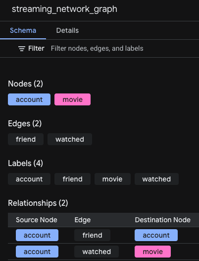
create graph streaming_service{
node account ({name string})
, node movie ({title string})
, edge watched (account)-[{watched_at datetime}]->(movie)
, edge friends (account)-[]->(account)
};
use streaming_service;
INSERT (n1:account {_id:'fatima', name:"Fatima"})
, (n2:account {_id:'maryam', name:"Maryam"})
, (n3:account {_id:'uroosa', name:"Uroosa"})
, (n4:account {_id:'sara', name:"Sara"})
, (n5:account {_id:'zainab', name:"Zainab"})
, (n6:account {_id:'hannah', name:"Hannah"})
, (m1:movie {_id:'time_hoppers', title:"Time Hoppers"})
, (m2:movie {_id:'despicable_me', title:"Despicable Me"})
, (m3:movie {_id:'penguins_of_madagascar', title:"Penguins of Madagascar"})
, (m4:movie {_id:'zootopia', title:"Zootopia"})
, (n1)-[:friends]->(n2)
, (n2)-[:friends]->(n1)
, (n2)-[:friends]->(n3)
, (n3)-[:friends]->(n2)
, (n3)-[:friends]->(n4)
, (n4)-[:friends]->(n3)
, (n5)-[:friends]->(n6)
, (n6)-[:friends]->(n5)
, (n1)-[:watched {watched_at: '2024-01-01T20:00:00Z'}]->(m1)
, (n1)-[:watched {watched_at: '2024-01-02T20:00:00Z'}]->(m2)
, (n2)-[:watched {watched_at: '2024-01-01T21:00:00Z'}]->(m1)
, (n3)-[:watched {watched_at: '2024-01-01T22:00:00Z'}]->(m3)
, (n4)-[:watched {watched_at: '2024-01-01T23:00:00Z'}]->(m4)
, (n5)-[:watched {watched_at: '2024-01-01T19:30:00Z'}]->(m1)
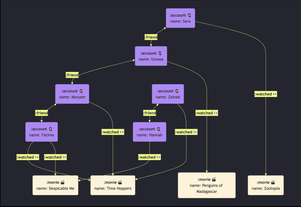
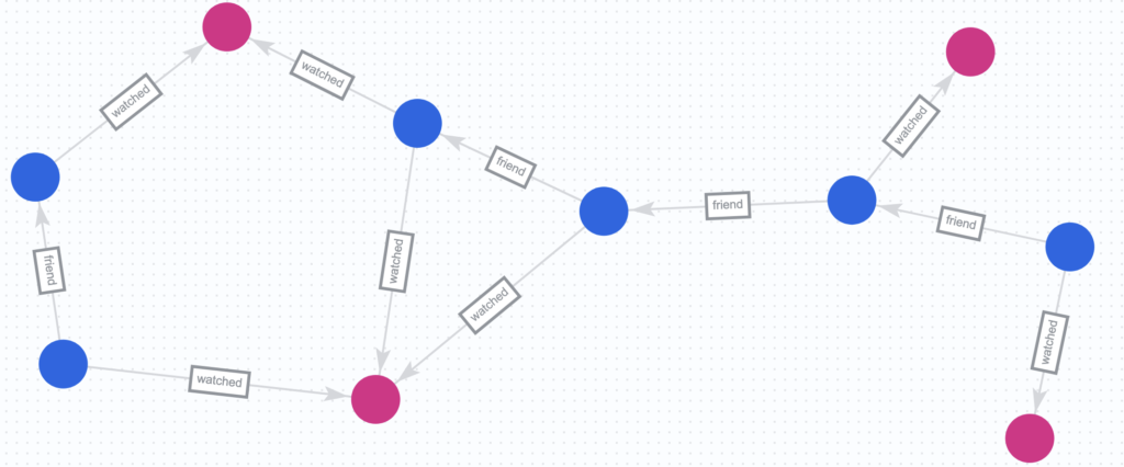
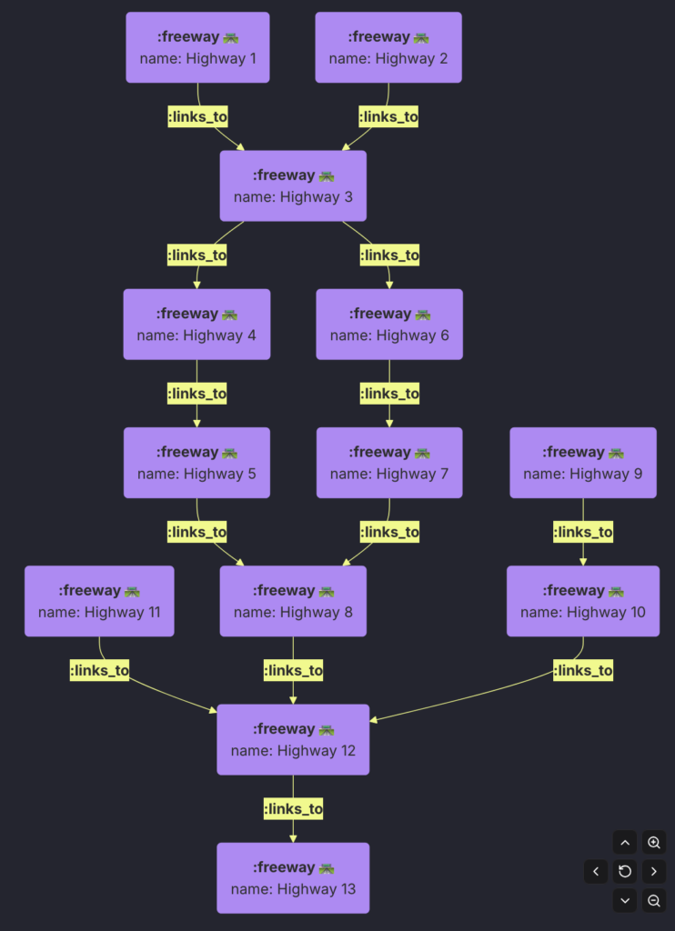
, (n6)-[:watched {watched_at: '2024-01-01T18:30:00Z'}]->(m2);This will create the following graph:
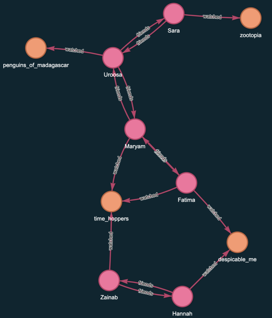
Now let’s write GQL query to get the recommendation for each person based on what their 1st and 2nd degree connections watched
MATCH friends = ALL (account_a)-[:friends]->{0,2}(account_b)
CALL {
MATCH path = (account_a)-[:watched]->(movie_a)
, (account_b)-[:watched]->(movie_b)
FILTER account_a <> account_b and movie_a <> movie_b
return path
, COLLECT_LIST(distinct movie_a.title) as recommended_movies
}
FILTER account_a <> account_b
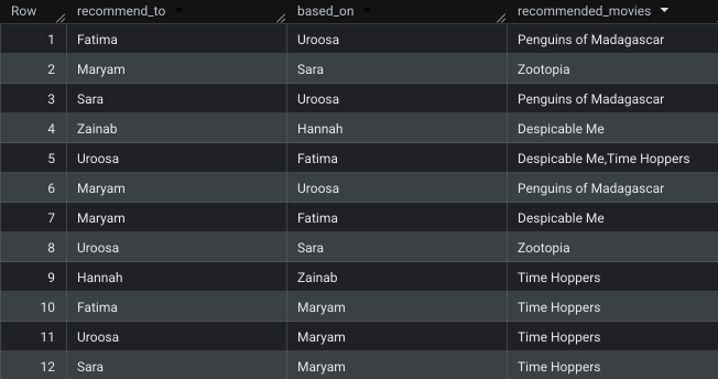
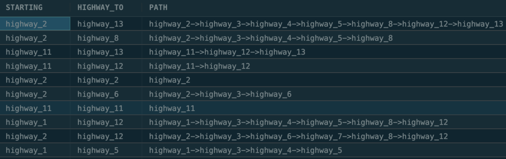
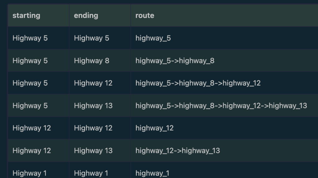
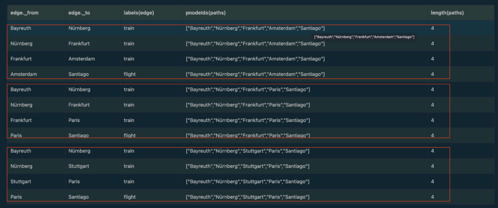
return table(account_b.name as recommend_to , account_a.name as based_on, recommended_movies);This will output
Note that we use the inline CALL function to iterate over each connections pair.